Pandas for Excel Monkeys

Because you don't want to do VBA.

• Introduction
  • Installation
  • Our Example Excel and CSV Files
  • Import Statement
• Loading Data
  • Loading a Specific Excel Sheet
  • Loading a CSV File
• Fixing Table Structure Problems
  • Wrong Column Names
  • Avoiding Column Names Altogether
  • Column Names Starting in a Different Row
  • Unwanted Rows
  • Wrong Column Types
  • Custom Column Conversion
• Saving Data
  • As CSV
  • As Excel (Single Sheet)
  • As Excel (Multiple Sheets)
• Manipulating a Sheet
  • Duplicating a DataFrame
  • Deleting Columns and Rows
  • Copy/Pasting
  • Sorting
  • Filtering (Blanks)
  • Filtering (By Value)
  • Filtering (By Expression)
• Functions
• Cell Range Selection
  • SUM, AVERAGE, AND MEDIAN
• Conclusion
  • Thanks

Introduction

I am an Excel monkey. What do monkeys have to do with pandas? If you are like me and tend to solve all problems that involve data and numerical calculation in Excel, you must have come across a dreaded moment in your life in which you had to decide between cleaning the data from scratch every time there was a change, writing a cryptic nested set of functions, or…. (drum roll) writing a VBA script. Of course, the moment the only way to solve a problem is by writing a VBA script, something has gone terribly wrong.

I refuse to do VBA. No, it is not because it is BASIC and I am elitist, I’ve spent most of my childhood writing BASIC programs after all. It is the fact that I have to learn a complete object model from scratch that bears no relationship with the experience at the function level. With Pandas we can be consistent and use the same object model with no discrimination between “beginner” and “expert mode”. In short, an Excel monkey like me (and you?) can use Pandas pretending it is Excel whilst having the luxury of living in a Python world if a more complicated problem arises.

In a nutshell, why should you migrate from Excel to Pandas?

1. Because you don’t want to import and clean new data sets manually every time there is a change
2. Becuase you still want instant gratification which Pandas provides when running on Jupyter Notebook
3. Because you want to use a humane programming language when you run into problems. You will not learn COBOL. You will not learn VBA.
4. Because I’ve written this tutorial to make the transition painless

To be blunt, this tutorial is written from an Excel user perspective. I’ve captured the use cases that apply to 80% of what I do in Excel; as such, I emphasise Excel terminology and I may violate some (if not all) of the idomatic patterns that Pandas users with PhDs abide to.

Installation

We first import the Pandas library which in turn uses numpy (typially retrieved automatically as a transitive dependency) and xlrd for reading Excel files which must be installed manually. This tutorial, in particular, has been written as a Jupyter Notebook and then exported as a markdown file, similarly to the workflow that I typically use with Literal Haskell in some of my other blog posts. As such, I also highly recommend installing Jupyter Notebook which is a must have to truly feel “at home”.

pip3 install pandas
pip3 install xlrd
pip3 install openpyxl
pip3 install jupyter

Our Example Excel and CSV Files

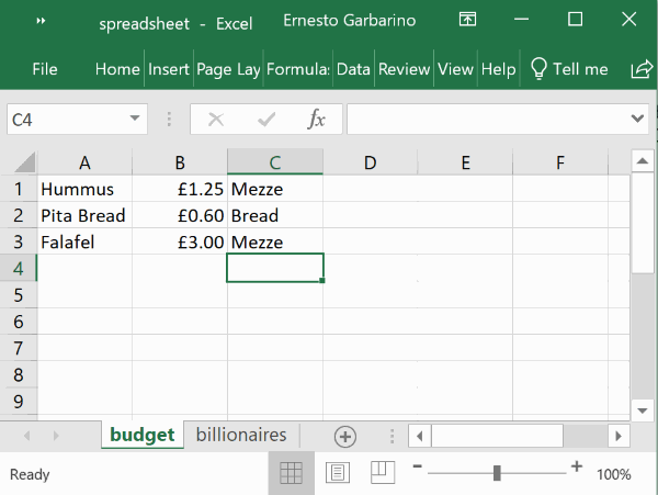
All of this tutorial is based on an Excel file called spreadsheet.xlsx that contains two sheets:

The same two sheets are also assumed to be available as separate CSV files: budget.csv and billionaires.csv.

Import Statement

We obviously need to first import the library so that we can make use of it. The NumPy import is necessary when referencing types (e.g. np.float64) which underpin Pandas’ objects.

import pandas as pd
import numpy  as np

Loading Data

Before we can manipulate data with Pandas, we need to load it. Data is typically loaded from Excel, CSV and SQL sources. Naturally, as this is a tutorial intended for Excel users (like the author) the focus will be on the first method.

Loading a Specific Excel Sheet

An Excel file, at at the top level, is a collection of sheets. Loading an “Excel file” actually means loading a specific sheet rather than set of them. Unless otherwise specified, the read_excel() method will read the first sheet by default:

pd.read_excel('spreadsheet.xlsx')

The file spreadsheet.xlsx contains two sheets, budget and billionaires. If we wanted to load the second sheet instead, we can specify it as the second argument that takes either the sheet’s name or an ordinal number:

pd.read_excel('spreadsheet.xlsx', 'billionaires')

pd.read_excel('spreadsheet.xlsx', 1)

Loading a CSV File

Comma Separated Value (CSV) files are expected to be like single sheets. In the example below, the read_csv() method behaves similarly to the Excel version. CSV files exported from Excel, on a Windows machine, are typically loaded successfully using latin1 as the value of the encoding parameter:

pd.read_csv('budget.csv', encoding='latin1')

pd.read_csv('billionaires.csv', encoding='latin1')

Fixing Table Structure Problems

Both Excel sheets and CSV files are loaded into an object type called a DataFrame. A DataFrame can be thought of as a SQL table that is defined as a set of named columns which store a given type (e.g. a String, an Integer, a Date, etc.). As we have seen in the above examples, the loaded data does not seem to be correct from a tabular representation (i.e. a DataFrame) perspective. This is on purpose. Let us fix those problems one at a time.

The additional arguments to be shown work both with the read_excel() and read_csv() functions.

Wrong Column Names

The sheet budget.csv lacks columns names which results in Pandas assuming that the first row represents the column labels:

pd.read_csv('budget.csv',encoding='latin1')

To correct this problem all we have to do is specify the column names by declaring the names argument which takes a list of column labels:

pd.read_csv('budget.csv',encoding='latin1',names=['Food Name','Price','Type'])

Avoiding Column Names Altogether

Sometimes we don’t want the hassle of specifying column names at all but we still want a well-formed DataFrame object. No problem, we just set the header argument to None which results in Pandas simply assigning an incremental integer to each column:

pd.read_csv('budget.csv',encoding='latin1',header=None)

Column Names Starting in a Different Row

The other problem we have seen is that column names may not be declared in row 0:

pd.read_csv('billionaires.csv',encoding='latin1')

The solution here is to specify the row number using the header argument:

pd.read_csv('billionaires.csv',encoding='latin1',header=1)

Unwanted Rows

It is customary for Excel users to recycle rows further down a table to add additional calculations such as the Average, Mean and Total functions as shown in our billionaires.csv sheet. Not only we don’t typically want to read such extra cells but they typically have types that violate the DataFrame structure. Each column (called a Series) should hold elements of the same type.

The simplest solution is just to specify the exact number of rows to be read using the nrows argument:

pd.read_csv('billionaires.csv',encoding='latin1',header=1,nrows=3)

Conversely, the skiprows argument may be used to start reading from a different row other than 0, but, as shown below, this may also skip the column that declares the column labels:

pd.read_csv('billionaires.csv',encoding='latin1',header=1,skiprows=1,nrows=2)

Wrong Column Types

Pandas will try to guess each column type but we may not be happy with its “educated” guess or we may simply want to cast the underlying value to a new type.

Column types are specified using the dtype argument whose value is a dictionary in which the keys are the column names (or indices) and the values are the desired Python/NumPy types.

In the below example, we change the column Age to float.

pd.read_csv('billionaires.csv',encoding='latin1',header=1,nrows=3,dtype={'Age' : float})

If we don’t know what type Pandas has assumed, we can just query the dtypes property:

df = pd.read_csv('billionaires.csv',encoding='latin1',header=1,nrows=3)
df.dtypes

Name          object
Age            int64
Net Worth    float64
dtype: object

A similar approach is the use of the info() function:

df.info()

<class ‘pandas.core.frame.DataFrame’> RangeIndex: 3 entries, 0 to 2 Data columns (total 3 columns): Name 3 non-null object Age 3 non-null int64 Net Worth 3 non-null float64 dtypes: float64(1), int64(1), object(1) memory usage: 152.0+ bytes

Custom Column Conversion

The use of the dtype argument is limited in that it forces a cast on the underlying type and it will fail if the information may be lost (e.g. casting a float down to an int). In such cases we need a custom conversion function which is provided using the converters argument. This argument is similar to dtype in the sense that it is a dictionary in which the keys are column names but the difference is that the argument is a custom conversion function as opposed to a type.

to_dollars = lambda x : "${:,.0f}".format(np.float64(x)*10**9)

pd.read_csv('billionaires.csv',encoding='latin1',header=1,nrows=3,
             converters={'Age' : (lambda x : str(x) + " years"),
                         'Net Worth' : to_dollars})

Saving Data

As we have seen before, data often needs to be cleaned before it is loaded. When saving data, what we are saving is actually a DataFrame object which contains multiple columns and rows. As such, we will use budget.csv as an example of a correct DataFrame:

df = pd.read_csv('budget.csv',encoding='latin1',names=['Food Name','Price','Type'])
df # display DataFrame

As CSV

Saving as CSV is simply a matter of using the to_csv() function.

df.to_csv('budget_fixed.csv')

However, unless otherwise specificed, the row number will be included as a value which is not typically what we want:

pd.read_csv('budget_fixed.csv')

To fix this problem, we just set the index argument to False:

df.to_csv('budget_fixed.csv',index=False)
pd.read_csv('budget_fixed.csv')

In the case of larger data sets, the use of actual commas (the , character) is undesirable. Tabs (represented by the \t escape code) are preferred since long fragments of text often contain commas. This or any other separator is specified using the sep argument. Some other typical use cases when exporting to CSV is the omission of the header columns which is enabled by setting header to False and the choice of a specific encoding using the encoding argument.

df.to_csv('budget_fixed.csv',index=False,header=False,sep='\t',encoding="utf-8")
pd.read_csv('budget_fixed.csv',sep='\t',header=None)

As Excel (Single Sheet)

The to_excel() function works similarly to the to_csv() one.

df.to_excel('budget_fixed.xlsx')
pd.read_excel('budget_fixed.xlsx')

It does seem like there’s nothing else to do but if we open the actual Excel file we will see row numbers on column A which we can prevent by adding the index=False argument. Another typical requirement is naming the sheet using sheet_name argument or adding a second argument:

df.to_excel('budget_fixed.xlsx','Budget',index=False)
pd.read_excel('budget_fixed.xlsx')

As Excel (Multiple Sheets)

Business people won’t tolerate the hassle of opening multiple different files just because that’s what a “Data Science” team produces. Saving multiple DataFrames as multiple sheets that are then combined in a single Excel document is just what the doctor ordered. The workflow here is slightly different.

To complete the example, we will be declaring a second DataFrame, df2 in which will load the list of billionaires:

df2 = pd.read_csv('billionaires.csv',encoding='latin1',header=1,nrows=3)
df2 # display DataFrame

Now, we have df (declared at the start of this section) that contains a budget items, and df2 that contains a list of billionaires. To save the two DataFrames as different named sheets in a file called combined.xlsx, we proceed as follows:

writer = pd.ExcelWriter('combined.xlsx')
df.to_excel(writer,'Budget', index=False)
df2.to_excel(writer,'Billionaires', index=False)
writer.save()

Manipulating a Sheet

So far we have learned how to get data into Pandas, how to fix some typical “import” problems and how to save the data back to a file. As part of these lessons we have also got used to the idea that a DataFrame is sort of the Pandas version of an Excel sheet.

df = pd.read_csv('budget.csv',encoding='latin1',names=['Food Name','Price'])
type(df)

pandas.core.frame.DataFrame

In Excel, before we apply any formula, we can do all sorts of manipulations at the sheet level such as ordering by a given column type, filtering by a given value and so on. This is exactly what we will do in this section.

Duplicating a DataFrame

It is common in Excel to create a copy of a sheet before we apply changes to it in case we do a mistake. We can do exactly the same thing with a DataFrame

df1 = pd.read_csv('billionaires.csv',encoding='latin1',header=1,nrows=3)
df2 = df1.copy()
df1.equals(df2)

True

Deleting Columns and Rows

The first thing we do in Excel after importing a data file is getting rid of the rows and columns we don’t want; to achieve this we just pass the columns and rows that we want to discard to the drop() function using the columns, and index arguments, respectively.

Original

df1

New DataFrame

# Drop returns a new DataFrame by default unless we add inplace=True
df1.drop(columns=['Age'],index=[1])

Copy/Pasting

An alternative approach to deleting rows and columns in Excel is simply selecting the data that we want and pasting it on a new sheet.

Original

df1 # display DataFrame

Copying Rows

# Slice syntax
df1.loc[1:] 

# Specific rows
df1.loc[[0,2]] 

Copying Columns

# Slice syntax 
df1.iloc[:,1:] 

# Specific columns
df1[['Name','Net Worth']]

Sorting

Sorting and filtering are Excel’s best known staple functions. The sort_values() function is Panda’s answer to our trusted “A->Z” Excel icon:

df1.sort_values('Net Worth')

Oh, there is also a “Z->A” icon too in Excel. This means, sort in descending, rather than ascending, order:

df1.sort_values('Net Worth',ascending=False)

Filtering (Blanks)

The innocent “Filter” funnel-looking icon in Excel provides a number of filtering strategies for each column but the ability to filter out blanks is such a common use case that Pandas also has an explicit approach to it. To illustrate the filtering of blanks, we will use the longer version of the billionaires sheet:

df2 = pd.read_csv('billionaires.csv',encoding='latin1',header=1)
df2 # display DataFrame

If all we want is just get rid of any rows that contain blanks, we simply call dropna() without any arguments:

df2.dropna()

Alternatively, we may want to get rid of the columns that contain blanks:

df2.dropna(axis='columns')

In Excel, though, we typically specify that we want rows to be removed only if blanks appear in given columns:

# note that 'Net Worth' has no blanks
df2.dropna(subset=['Age', 'Net Worth'])

Filtering (By Value)

Filtering by value in Excel comes with the added benefit that we are presented with a summary of all unique values present in a given column. Obviously, we need to find out how to do this in Pandas first, before we select a value. For this illustration, we’ll revert back to the budget.csv sheet:

df = pd.read_csv('budget.csv',encoding='latin1',names=['Name','Price','Type'])
df # display DataFrame

Here we want to apply a “filter” on the column Type but before we need to find out what unique values are in Type:

df['Type'].unique()

array(['Mezze', 'Bread'], dtype=object)

So let’s filter column Type by selecting the Mezze value

df[df['Type'] == 'Mezze']

Filtering (By Expression)

Filtering by expression is actually the same as filtering by value. We presented this as a separate approach simply to align with the Excel workflow. Most Excel users don’t bother with custom filtering expressions since filtering by blanks or unique values is sufficient. Here is an example:

df # display DataFrame

df[df['Price'] > 1.0]

Functions

The whole point of using a spreadsheet is performing calculations. So far, all we’ve done is just manipulate and query a tabular structure. In Excel, we can do local calculations such as =2*3 but the interesting thing is applying functions to the contents of cells and cell ranges.

Cell Range Selection

The result of a cell range selection in Pandas is stored in a object of type Series that, like DataFrames, has several functions. First, let us pick up again a reference DataFrame:

df = pd.read_csv('billionaires.csv',encoding='latin1',header=1,nrows=3)
df # display DataFrame

A single value, like Warren Buffet is referenced in an Excel-esque manner by simply indicating its row number and column:

df.loc[0,'Name']

'Warren Buffet'

A “cell range” selection depends on whether we want columns or rows, and whether we want the entire set or a “delimited” one.

Selecting Cells within Columns

# Select all 'cells' in the Age column
df['Age']

0    88
1    63
2    54
Name: Age, dtype: int64

# Select the second and third cells in 'Age'
df['Age'][1:3]

1    63
2    54
Name: Age, dtype: int64

Selecting Cells within Rows

# Select all 'cells' in the first row
df.loc[0]

Name         Warren Buffet
Age                     88
Net Worth             84.4
Name: 0, dtype: object

# Select the first and second cells from the first row
df.loc[0][0:2]

Name    Warren Buffet
Age                88
Name: 0, dtype: object

SUM, AVERAGE, AND MEDIAN

Although there is no printf() in Excel, most people would not disagree that writing the first =SUM() function would be the nearest equivalent of “Hello World”. Naturally, =AVERAGE() and =MEDIAN() come next.

Let us refresh our minds again about the contents of df because we are all forgetful:

df = pd.read_csv('billionaires.csv',encoding='latin1',header=1,nrows=3)
df # display DataFrame

And now let Pandas makes us feel at home

df['Net Worth'].sum()

318.70000000000005

df['Net Worth'].mean()

106.23333333333335

df['Net Worth'].median()

96.7

Conclusion

We have learned how to load and save data files, how to order and select data, and how to perform some basic calculations, using Pandas. Although this is the tip of the iceberg, in terms of what Panda offers, the acquired skills should be sufficient for someone who is both familiar with Excel and Python to make the transition. Most importantly, a problem that would be typically be solved in VBA can bow be taken to Python and back to Excel again with no fuzz.

Thanks

• Ben Simonds for introducing me to Jupyter Notebook
• Shanghai Daily for the cover picture